


zkVM (Zero-Knowledge Virtual Machine) is a virtual machine that utilizes Zero-Knowledge Proofs (ZKP) to ensure the correctness, integrity, and privacy of computations.
Zero-Knowledge Proof: A proof where the prover demonstrates to the verifier that a statement is true, without revealing any information beyond the truth of the statement. It includes the following four properties:
Validity Proof:
Fraud Proof:
Verifiable Computation:
When writing a ZKP application, the following three steps are involved:

Here is an example of how to implement a multiplier using Circom.
Multiplier2.circom:
pragma circom 2.0.0;
/* This circuit template checks if c is the product of a and b. */
template Multiplier2 () {
   // Signal declarations
   signal input a;
   signal input b;
   signal output c;
   // Constraints
   c <== a * b;
}
The flowchart is as follows:

Arithmetization: Converting a program into a set of polynomials
Circuit Computation:
This method reduces the program to the gate-level concept. However, the gates here are not physical gates in a processor, but logical concept gates.
R1CS: The maximum polynomial degree is 2, satisfying the following equation:
\[\left(\sum_{k}A_{ik}Z_{k}\right)\left(\sum_{k}B_{ik}Z_{k}\right)-\left(\sum_{k}C_{ik}Z_{k}\right)=0\]
Where \(A_{ik'}, B_{ik'}, C_{ik}\) are elements from a finite field F. For example, the expression \(y = x^3\) can be represented by introducing intermediate variables as follows:
\[x \cdot x = w_1\]\[w_1 \cdot w_1 = w\]
Intermediate variables can be private or public inputs of the circuit. It is important to note that the R1CS representation of a computation is not unique. For example, the above expression could also be represented as:
\[x \cdot x = w_1\]\[w_1 \cdot x = w_2\]\[w_2 \cdot x = w_3\]
Plonkish: Supports two-input gates (two fan-in gates), allowing for the implementation of custom gates.
\[q_{L}x_{a}+q_{R}x_{b}+q_{o}x_{c}+q_{M}x_{a}x_{b}+q_{c}=0\]
Where \(q_{L}, q_{R}, q_{O}, q_{M}, q_{C}\) are control parameters for the selection operations, used to represent R1CS operations.
Computational Computation:
This method is similar to how computers work, involving a set of registers and state transition functions that modify the register values.
AIR and PAIR: Suitable for uniform computations.


The Fiat-Shamir method can be used to convert the interactive protocol into a non-interactive one.


Commitment Phase
The prover \(P\) submits a polynomial \(p_0\) over a multiplicative subgroup \(H\). The degree of the polynomial is \(d\), and all elements come from the field \(F\), where \(G\) is the generator of field \(F\), and \(K\) is the extension field of \(H\).
MTR is the root node of the Merkle tree. The verifier randomly generates a value and sends it to the prover, who then submits the MTR to the verifier as the opening value.

Proof Systems:
Publish Verifier on-chain:
Question: Can we use high-level languages (such as Golang, Rust) to define problem models?

In computing, a virtual machine (VM) is a virtualization or simulation of a computer system. A virtual machine is based on computer architecture and provides functionality similar to a physical computer.
Computer Architecture refers to the structure of a computer system composed of components like CPU, memory, ALU, etc.

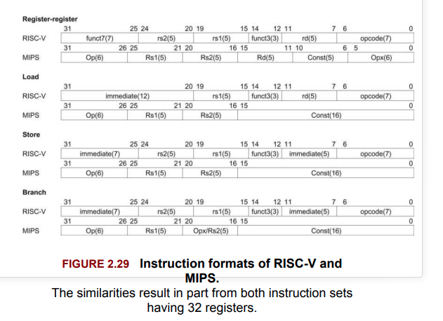
RISC (Reduced Instruction Set Computer) is designed to simplify the instruction set used by computers when performing tasks.
Below is an example of the ADDI instruction in MIPS32, which allows for the selection of a source register, a target register, and includes a small constant.

In zkVM, there are three main RISC ISAs:
Among them, RISC V is similar to a simplified version of MIPS.
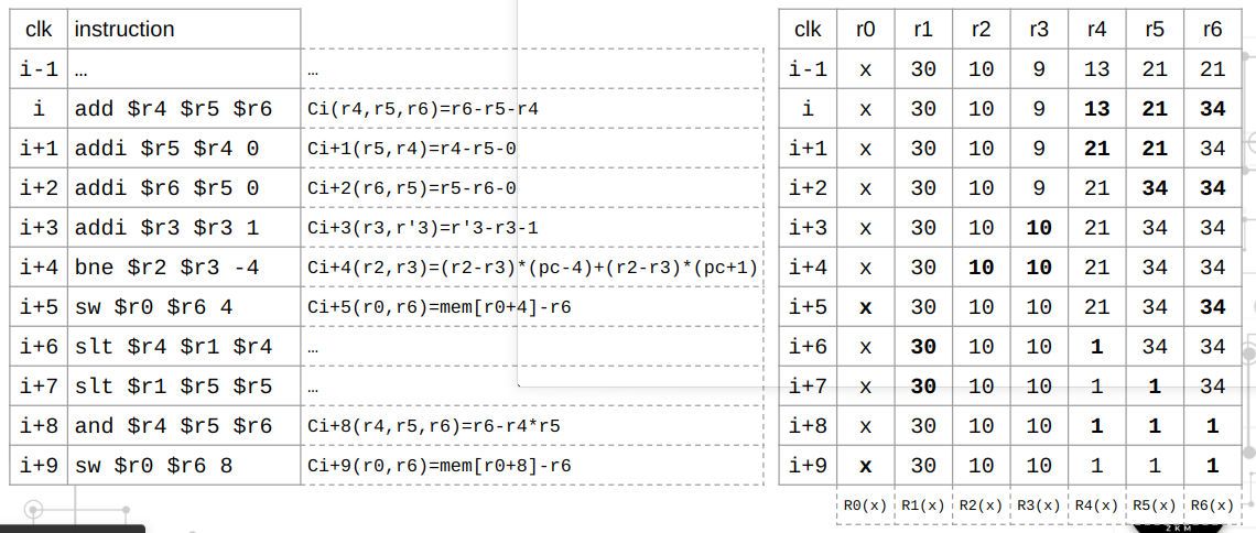
Based on existing knowledge, we can implement a simple zkVM, such as a Fibonacci executor, to calculate the n-th term of the Fibonacci sequence.
\[f(n) = f(n-1) + f(n-2) \quad f(0) = f(1) = 1\]
We choose AIR (Algebraic Intermediate Representation) as the algebraization method.
Define a state machine \(S\) containing the following two variables, and let \(i\) be the field size:
\[S = (A_i, B_i) \quad S' = (A_{i+1}, B_{i+1})\]
Now, the state machine S can represent the Fibonacci executor as follows:
\[A_{i+1} = B_i \quad B_{i+1} = A_i + B_i\]
Thus, for all \(i\) in the field, the execution trace table is as follows, where \(n = 6\):

In the virtual machine, each state is represented by a register.
The polynomials representing two registers come from the polynomial set \(F_p[X]\), where the coefficients are elements from the prime field \(F_p\) and \(p = 2^{64} - 2^{32} + 1\)
Thus, the domain forms a subgroup:
\[H = \{\omega_0, \omega_1, \omega_2, ..., \omega_d = \omega_0\} \subset F_p^d\]
Define two polynomials \(P(X)\) and \(Q(X)\) to represent the trace columns A and B:
\[P(\omega^{i})=A_{i}Q(\omega^{i})=B_{i}\]
It is clear that:
\[P(\omega^{i}\cdot\omega)=P(\omega^{i+1})=A_{i+1}\]
\[Q(\omega^{i}\cdot\omega)=Q(\omega^{i+1})=B_{i+1}\]
Using Lagrange interpolation, we can compute the coefficient form of \(P\) and \(Q\).
Now, we can use polynomial constraints to limit the state transitions with two registers:
\[P(X \cdot \omega) = I_H Q(X)\]
\[Q(X \cdot \omega) = I_H P(X) + Q(X)\]
Since \(H\) is a subgroup, we have:
\[P(\omega^{5}\cdot\omega)=I_{H}Q(\omega^{5})=13\]
\[P(\omega^{5}\cdot\omega)=P(\omega^{0})=1\]
Clearly, the constraint is broken in the last row.
The solution is to introduce another register LAST to mark the last row and assign it a vector value \([0, ..., 1]\). The trace table becomes:
\[P(X \cdot \omega) = I_H Q(X) \cdot (1 - \text{LAST}(X)) + \text{LAST}(X) \cdot P(\omega^0)\]
\[Q(X \cdot \omega) = I_H (P(X) + Q(X)) \cdot (1 - \text{LAST}(X)) + \text{LAST}(X)\]
In summary, there are two basic types of constraints in the state machine:
In actual zkVM development, there are various types of instructions, such as arithmetic, logical, branching/jumping, and memory operations. Each instruction requires only a small amount of state to represent, but a program may require thousands of states.
Below is an overview of the zkMIPS implementation:

Now, the constraints mentioned above can be transformed into polynomial equalities:
\[P_0 = (1 - \text{LAST}(X)) \cdot (P(X \cdot \omega) - Q(X)) = 0\]
\[P_1 = (1 - \text{LAST}(X)) \cdot (Q(X \cdot \omega) - (P(X) + Q(X))) = 0\]
The proof system based on polynomial equalities utilizes the fundamental properties of the Schwartz-Zippel Lemma.
According to the Schwartz-Zippel Lemma, the probability that the prover finds a false polynomial Q' (with degree d) that satisfies:
\[Q'(\alpha_j) = Q(\alpha_j) \quad \text{for all } j \in \{1, 2, ..., l\}\]
for random challenges \(\{\alpha_1, \alpha_2, ..., \alpha_i\}\) from the verifier is at most \(\frac{d}{|S|}\), which is negligible.
Define \(z_H(X)\) as the vanishing polynomial, and compute the quotient polynomials \(q_i(X)\):
\[P_0 = (1 - \text{LAST}(X)) \cdot (P(X \cdot \omega) - Q(X)) = z_H(X) \cdot q_i(X)\]
\[P_1 = (1 - \text{LAST}(X)) \cdot (Q(X \cdot \omega) - (P(X) + Q(X)))\]
Therefore, we can use polynomial commitment schemes (such as FRI or KZG) to commit to the trace and quotient polynomials \(R_i, q_i(X)\).
Generally, there are three main types of zkVMs:

Taking zkMIPS as an example, we have implemented 62 instructions and categorized them as follows:
Thus, if we use a single trace table and place all state variables in it, the table becomes very large and sparse (i.e., many zero-value entries). This leads to the following issues:
Both of these points lead to a substantial computational load in the Polynomial Commitment Scheme (PCS).
A common optimization method is to split the large table into multiple sub-tables, as shown below:

This splitting brings additional engineering benefits:
Lookup arguments allow proof that the vector elements submitted by the prover come from another (larger) committed table. Such schemes are commonly used to implement the communication bus in zkVMs. Broadly speaking, these protocols can be used to prove statements of the following form:
In this framework, the table \(T\) is typically considered public, and the lookup list \(F\) is treated as private evidence. Table \(T\) can be understood as storing all valid values for a particular variable, while the lookup list \(F\) contains the specific instances of this variable generated during program execution. The proven statement asserts that throughout program execution, the variable always remains within its valid range.
In this discussion, we assume \(m < N\), and typically \(m \ll N\) (unless stated otherwise). We will review the evolution of lookup protocols and their various applications.
Before delving into lookup schemes, let’s first examine a permutation parameter using multiset equality:
\[\prod_{i}(X-f_{i})=\prod_{j}(X-t_{j})\]
where \(X\) belongs to the field \(F\). We can choose a random number \(\alpha \in F\) and simplify the check of the above polynomial equality into a grand product.
Moreover, if \(F \subseteq T\), there exists \(m_j\) such that:
\[\prod_{i}(x-f_{i})=\prod_{j}(x-t_{j})^{m_{j}}\]
In particular, if all \(m_j\) are 1, then we have a multiset equality problem. This may seem to solve the problem, but the computational complexity is related to the size of set \(T\), which could be very large.
Let us now dive deeper into the history of lookup schemes.
Plookup is one of the earliest lookup protocols. The prover’s computational complexity is \(O(N \log N)\) field operations, and the protocol can be generalized to support multi-table and vector lookups. The process involves sorting the elements of vector f and table t in ascending order and defining:
\[\{(s_{k'},s_{k+1})\}=\{(t_{i},t_{j+1})\}\cup\{(f_{i},f_{i+1})\}\]
as multisets, and then performing the following check:
\[\prod_{k}(X+s_{k}+Y\cdot s_{k+1})=\prod_{i}(X+f_{i}+Y\cdot f_{i+1})\prod_{j}(X+t_{j}+Y\cdot t_{j+1})\]
where \(X\) and \(Y\) belong to the field \(F\).
This protocol can be simplified further using a grand product.
Caulk makes the prover’s workload dependent on the size \(m\) of \(C_{M}\) rather than the size \(N\) of \(C\). The prover identifies a subset \(C_{i}\) (which contains elements of \(C_{M}\)) and uses a KZG commitment to prove that \(C - C_i = Z_i(x) \cdot H_i(x)\). This protocol has sublinear efficiency, with a prover complexity of \(O(m \log N)\).
Caulk+ is an improved version of Caulk that reduces the prover’s computational complexity further by more efficient divisibility checks. The protocol proves that \(Z_i\) can divide \(C - C_i\) and \(x^n - 1\) by computing the polynomials \(Z_{I}\), \(C_{i}\), and \(U\). With the introduction of blinding factors to preserve zero-knowledge properties, the prover’s complexity is reduced to \(O(m^2)\).
Baloo extends Caulk+ by committing to subsets of the table in the form of vanishing polynomials, achieving nearly linear time complexity for the subset size. It introduces a “commit and prove” protocol and uses the general Sumcheck protocol to reduce the proof to an inner product argument. This protocol is efficient and supports multi-column lookups, showing wide applicability in SNARKs such as zkEVM.
Flookup is designed for efficiently proving that the value of a committed polynomial belongs to a large table. The protocol leverages pairings to extract vanishing polynomials for related table subsets and introduces a new interactive proof system (IOP). After \(O(N \log^2 N)\) preprocessing, the prover operates in nearly linear time \(O(m \log^2 m)\), offering substantial improvements over previous quadratic complexities, particularly for SNARKs over large fields.
cq uses logarithmic derivative methods to simplify membership proofs to rational polynomial equality checks. By precomputing cached quotients for quotient polynomials, the protocol makes table item computations more efficient. The prover time is \(O(N \log N)\), and the proof size is \(O(N)\), offering better efficiency than Baloo and Flookup while maintaining homomorphic properties.
LogUp efficiently proves that a set of witness values exists within a Boolean hypercube lookup table. By using logarithmic derivatives, this method transforms the set inclusion problem into rational function equality checks, requiring the prover to provide only a multiplicity function. LogUp is more efficient than multi-variable Plookup variants, requiring 3-4 times fewer Oracle commitments. For large-scale lookups, its efficiency also surpasses the bounded multiplicity optimization of Plookup. This method is well-suited for vector-valued lookups and scalable for range proofs, playing a crucial role in SNARKs (such as PLONK and Aurora) and applications like tinyRAM and zkEVM.
Further reading: Lookup Protocol Paper and Video Link
Aggregation is the simplest way to generate individual proofs for each block and combine them into another proof. The first type of proof verifies “the block is valid and on-chain”, while the second type verifies “all these block proofs are valid.” This method is known as aggregation.
In an aggregation scheme, the second circuit can only start aggregation after all block proofs are ready. However, what if we could process the blocks one by one? This is what recursion accomplishes.
In a recursive scheme, each block proof verifies two things: the current block is valid, and the previous proof is valid. One proof “wraps” the previous proof, with the overall structure resembling a chain.

Continuation is a mechanism for splitting a large program into smaller segments that can be executed and proven independently. This mechanism provides the following benefits:
Segment: A segment is a sequence of MIPS traces with entry PC and image ID.
Check Memory Consistency

To estimate the time required to generate a proof for program \(P\), we need to consider:
And use the following formula to calculate the ISA efficiency:
\[\text{#Instructions} \times \frac{\text{Constraint Complexity}}{\text{Per Instruction}} \times \frac{\text{Time}}{\text{Constraint Complexity}}\]
Source: Video Link
Method for Evaluating zkVM Performance:
Test scenarios: SHA2, SHA3, Rust EVM, Rust Tendermint, etc.
Metrics:
Open Source Frameworks:
Including RISCZero, zkMIPS, SP1, and Jolt, with benchmarks available at zkMIPS/zkvm-benchmarks.
zkVM should provide a developer-friendly toolchain that allows developers to build, compile their programs, and deploy validators onto the blockchain.
Correctness
The VM must execute programs as expected.
The proof system must meet its stated security properties, such as:
Conciseness
Hybrid Rollup: Optimistic + ZK
Metis combines the flexibility and composability of Optimistic Rollups with the scalability of zkMIPS to form a unified protocol, reducing final confirmation time from 7 days to less than 1 hour.
Bitcoin L2:
The GOAT network implements a BitVM2 protocol based on zkMIPS, building a truly secure Bitcoin L2.
zk Identity (zkIdentity)
zk Machine Learning (zkML)
Subscribe to the ZKM Blog to stay updated with the latest research by ZKM. If you have any questions about the article, you can contact the ZKM team on discord: discord.com/zkm
zkVM (Zero-Knowledge Virtual Machine) is a virtual machine that utilizes Zero-Knowledge Proofs (ZKP) to ensure the correctness, integrity, and privacy of computations.
Zero-Knowledge Proof: A proof where the prover demonstrates to the verifier that a statement is true, without revealing any information beyond the truth of the statement. It includes the following four properties:
Validity Proof:
Fraud Proof:
Verifiable Computation:
When writing a ZKP application, the following three steps are involved:
Here is an example of how to implement a multiplier using Circom.
Multiplier2.circom:
pragma circom 2.0.0;
/* This circuit template checks if c is the product of a and b. */
template Multiplier2 () {
   // Signal declarations
   signal input a;
   signal input b;
   signal output c;
   // Constraints
   c <== a * b;
}
The flowchart is as follows:
Arithmetization: Converting a program into a set of polynomials
Circuit Computation:
This method reduces the program to the gate-level concept. However, the gates here are not physical gates in a processor, but logical concept gates.
R1CS: The maximum polynomial degree is 2, satisfying the following equation:
\[\left(\sum_{k}A_{ik}Z_{k}\right)\left(\sum_{k}B_{ik}Z_{k}\right)-\left(\sum_{k}C_{ik}Z_{k}\right)=0\]
Where \(A_{ik'}, B_{ik'}, C_{ik}\) are elements from a finite field F. For example, the expression \(y = x^3\) can be represented by introducing intermediate variables as follows:
\[x \cdot x = w_1\]\[w_1 \cdot w_1 = w\]
Intermediate variables can be private or public inputs of the circuit. It is important to note that the R1CS representation of a computation is not unique. For example, the above expression could also be represented as:
\[x \cdot x = w_1\]\[w_1 \cdot x = w_2\]\[w_2 \cdot x = w_3\]
Plonkish: Supports two-input gates (two fan-in gates), allowing for the implementation of custom gates.
\[q_{L}x_{a}+q_{R}x_{b}+q_{o}x_{c}+q_{M}x_{a}x_{b}+q_{c}=0\]
Where \(q_{L}, q_{R}, q_{O}, q_{M}, q_{C}\) are control parameters for the selection operations, used to represent R1CS operations.
Computational Computation:
This method is similar to how computers work, involving a set of registers and state transition functions that modify the register values.
AIR and PAIR: Suitable for uniform computations.
The Fiat-Shamir method can be used to convert the interactive protocol into a non-interactive one.
Commitment Phase
The prover \(P\) submits a polynomial \(p_0\) over a multiplicative subgroup \(H\). The degree of the polynomial is \(d\), and all elements come from the field \(F\), where \(G\) is the generator of field \(F\), and \(K\) is the extension field of \(H\).
MTR is the root node of the Merkle tree. The verifier randomly generates a value and sends it to the prover, who then submits the MTR to the verifier as the opening value.
Proof Systems:
Publish Verifier on-chain:
Question: Can we use high-level languages (such as Golang, Rust) to define problem models?
In computing, a virtual machine (VM) is a virtualization or simulation of a computer system. A virtual machine is based on computer architecture and provides functionality similar to a physical computer.
Computer Architecture refers to the structure of a computer system composed of components like CPU, memory, ALU, etc.
RISC (Reduced Instruction Set Computer) is designed to simplify the instruction set used by computers when performing tasks.
Below is an example of the ADDI instruction in MIPS32, which allows for the selection of a source register, a target register, and includes a small constant.
In zkVM, there are three main RISC ISAs:
Among them, RISC V is similar to a simplified version of MIPS.
Based on existing knowledge, we can implement a simple zkVM, such as a Fibonacci executor, to calculate the n-th term of the Fibonacci sequence.
\[f(n) = f(n-1) + f(n-2) \quad f(0) = f(1) = 1\]
We choose AIR (Algebraic Intermediate Representation) as the algebraization method.
Define a state machine \(S\) containing the following two variables, and let \(i\) be the field size:
\[S = (A_i, B_i) \quad S' = (A_{i+1}, B_{i+1})\]
Now, the state machine S can represent the Fibonacci executor as follows:
\[A_{i+1} = B_i \quad B_{i+1} = A_i + B_i\]
Thus, for all \(i\) in the field, the execution trace table is as follows, where \(n = 6\):
In the virtual machine, each state is represented by a register.
The polynomials representing two registers come from the polynomial set \(F_p[X]\), where the coefficients are elements from the prime field \(F_p\) and \(p = 2^{64} - 2^{32} + 1\)
Thus, the domain forms a subgroup:
\[H = \{\omega_0, \omega_1, \omega_2, ..., \omega_d = \omega_0\} \subset F_p^d\]
Define two polynomials \(P(X)\) and \(Q(X)\) to represent the trace columns A and B:
\[P(\omega^{i})=A_{i}Q(\omega^{i})=B_{i}\]
It is clear that:
\[P(\omega^{i}\cdot\omega)=P(\omega^{i+1})=A_{i+1}\]
\[Q(\omega^{i}\cdot\omega)=Q(\omega^{i+1})=B_{i+1}\]
Using Lagrange interpolation, we can compute the coefficient form of \(P\) and \(Q\).
Now, we can use polynomial constraints to limit the state transitions with two registers:
\[P(X \cdot \omega) = I_H Q(X)\]
\[Q(X \cdot \omega) = I_H P(X) + Q(X)\]
Since \(H\) is a subgroup, we have:
\[P(\omega^{5}\cdot\omega)=I_{H}Q(\omega^{5})=13\]
\[P(\omega^{5}\cdot\omega)=P(\omega^{0})=1\]
Clearly, the constraint is broken in the last row.
The solution is to introduce another register LAST to mark the last row and assign it a vector value \([0, ..., 1]\). The trace table becomes:
\[P(X \cdot \omega) = I_H Q(X) \cdot (1 - \text{LAST}(X)) + \text{LAST}(X) \cdot P(\omega^0)\]
\[Q(X \cdot \omega) = I_H (P(X) + Q(X)) \cdot (1 - \text{LAST}(X)) + \text{LAST}(X)\]
In summary, there are two basic types of constraints in the state machine:
In actual zkVM development, there are various types of instructions, such as arithmetic, logical, branching/jumping, and memory operations. Each instruction requires only a small amount of state to represent, but a program may require thousands of states.
Below is an overview of the zkMIPS implementation:
Now, the constraints mentioned above can be transformed into polynomial equalities:
\[P_0 = (1 - \text{LAST}(X)) \cdot (P(X \cdot \omega) - Q(X)) = 0\]
\[P_1 = (1 - \text{LAST}(X)) \cdot (Q(X \cdot \omega) - (P(X) + Q(X))) = 0\]
The proof system based on polynomial equalities utilizes the fundamental properties of the Schwartz-Zippel Lemma.
According to the Schwartz-Zippel Lemma, the probability that the prover finds a false polynomial Q' (with degree d) that satisfies:
\[Q'(\alpha_j) = Q(\alpha_j) \quad \text{for all } j \in \{1, 2, ..., l\}\]
for random challenges \(\{\alpha_1, \alpha_2, ..., \alpha_i\}\) from the verifier is at most \(\frac{d}{|S|}\), which is negligible.
Define \(z_H(X)\) as the vanishing polynomial, and compute the quotient polynomials \(q_i(X)\):
\[P_0 = (1 - \text{LAST}(X)) \cdot (P(X \cdot \omega) - Q(X)) = z_H(X) \cdot q_i(X)\]
\[P_1 = (1 - \text{LAST}(X)) \cdot (Q(X \cdot \omega) - (P(X) + Q(X)))\]
Therefore, we can use polynomial commitment schemes (such as FRI or KZG) to commit to the trace and quotient polynomials \(R_i, q_i(X)\).
Generally, there are three main types of zkVMs:
Taking zkMIPS as an example, we have implemented 62 instructions and categorized them as follows:
Thus, if we use a single trace table and place all state variables in it, the table becomes very large and sparse (i.e., many zero-value entries). This leads to the following issues:
Both of these points lead to a substantial computational load in the Polynomial Commitment Scheme (PCS).
A common optimization method is to split the large table into multiple sub-tables, as shown below:
This splitting brings additional engineering benefits:
Lookup arguments allow proof that the vector elements submitted by the prover come from another (larger) committed table. Such schemes are commonly used to implement the communication bus in zkVMs. Broadly speaking, these protocols can be used to prove statements of the following form:
In this framework, the table \(T\) is typically considered public, and the lookup list \(F\) is treated as private evidence. Table \(T\) can be understood as storing all valid values for a particular variable, while the lookup list \(F\) contains the specific instances of this variable generated during program execution. The proven statement asserts that throughout program execution, the variable always remains within its valid range.
In this discussion, we assume \(m < N\), and typically \(m \ll N\) (unless stated otherwise). We will review the evolution of lookup protocols and their various applications.
Before delving into lookup schemes, let’s first examine a permutation parameter using multiset equality:
\[\prod_{i}(X-f_{i})=\prod_{j}(X-t_{j})\]
where \(X\) belongs to the field \(F\). We can choose a random number \(\alpha \in F\) and simplify the check of the above polynomial equality into a grand product.
Moreover, if \(F \subseteq T\), there exists \(m_j\) such that:
\[\prod_{i}(x-f_{i})=\prod_{j}(x-t_{j})^{m_{j}}\]
In particular, if all \(m_j\) are 1, then we have a multiset equality problem. This may seem to solve the problem, but the computational complexity is related to the size of set \(T\), which could be very large.
Let us now dive deeper into the history of lookup schemes.
Plookup is one of the earliest lookup protocols. The prover’s computational complexity is \(O(N \log N)\) field operations, and the protocol can be generalized to support multi-table and vector lookups. The process involves sorting the elements of vector f and table t in ascending order and defining:
\[\{(s_{k'},s_{k+1})\}=\{(t_{i},t_{j+1})\}\cup\{(f_{i},f_{i+1})\}\]
as multisets, and then performing the following check:
\[\prod_{k}(X+s_{k}+Y\cdot s_{k+1})=\prod_{i}(X+f_{i}+Y\cdot f_{i+1})\prod_{j}(X+t_{j}+Y\cdot t_{j+1})\]
where \(X\) and \(Y\) belong to the field \(F\).
This protocol can be simplified further using a grand product.
Caulk makes the prover’s workload dependent on the size \(m\) of \(C_{M}\) rather than the size \(N\) of \(C\). The prover identifies a subset \(C_{i}\) (which contains elements of \(C_{M}\)) and uses a KZG commitment to prove that \(C - C_i = Z_i(x) \cdot H_i(x)\). This protocol has sublinear efficiency, with a prover complexity of \(O(m \log N)\).
Caulk+ is an improved version of Caulk that reduces the prover’s computational complexity further by more efficient divisibility checks. The protocol proves that \(Z_i\) can divide \(C - C_i\) and \(x^n - 1\) by computing the polynomials \(Z_{I}\), \(C_{i}\), and \(U\). With the introduction of blinding factors to preserve zero-knowledge properties, the prover’s complexity is reduced to \(O(m^2)\).
Baloo extends Caulk+ by committing to subsets of the table in the form of vanishing polynomials, achieving nearly linear time complexity for the subset size. It introduces a “commit and prove” protocol and uses the general Sumcheck protocol to reduce the proof to an inner product argument. This protocol is efficient and supports multi-column lookups, showing wide applicability in SNARKs such as zkEVM.
Flookup is designed for efficiently proving that the value of a committed polynomial belongs to a large table. The protocol leverages pairings to extract vanishing polynomials for related table subsets and introduces a new interactive proof system (IOP). After \(O(N \log^2 N)\) preprocessing, the prover operates in nearly linear time \(O(m \log^2 m)\), offering substantial improvements over previous quadratic complexities, particularly for SNARKs over large fields.
cq uses logarithmic derivative methods to simplify membership proofs to rational polynomial equality checks. By precomputing cached quotients for quotient polynomials, the protocol makes table item computations more efficient. The prover time is \(O(N \log N)\), and the proof size is \(O(N)\), offering better efficiency than Baloo and Flookup while maintaining homomorphic properties.
LogUp efficiently proves that a set of witness values exists within a Boolean hypercube lookup table. By using logarithmic derivatives, this method transforms the set inclusion problem into rational function equality checks, requiring the prover to provide only a multiplicity function. LogUp is more efficient than multi-variable Plookup variants, requiring 3-4 times fewer Oracle commitments. For large-scale lookups, its efficiency also surpasses the bounded multiplicity optimization of Plookup. This method is well-suited for vector-valued lookups and scalable for range proofs, playing a crucial role in SNARKs (such as PLONK and Aurora) and applications like tinyRAM and zkEVM.
Further reading: Lookup Protocol Paper and Video Link
Aggregation is the simplest way to generate individual proofs for each block and combine them into another proof. The first type of proof verifies “the block is valid and on-chain”, while the second type verifies “all these block proofs are valid.” This method is known as aggregation.
In an aggregation scheme, the second circuit can only start aggregation after all block proofs are ready. However, what if we could process the blocks one by one? This is what recursion accomplishes.
In a recursive scheme, each block proof verifies two things: the current block is valid, and the previous proof is valid. One proof “wraps” the previous proof, with the overall structure resembling a chain.
Continuation is a mechanism for splitting a large program into smaller segments that can be executed and proven independently. This mechanism provides the following benefits:
Segment: A segment is a sequence of MIPS traces with entry PC and image ID.
Check Memory Consistency
To estimate the time required to generate a proof for program \(P\), we need to consider:
And use the following formula to calculate the ISA efficiency:
\[\text{#Instructions} \times \frac{\text{Constraint Complexity}}{\text{Per Instruction}} \times \frac{\text{Time}}{\text{Constraint Complexity}}\]
Source: Video Link
Method for Evaluating zkVM Performance:
Test scenarios: SHA2, SHA3, Rust EVM, Rust Tendermint, etc.
Metrics:
Open Source Frameworks:
Including RISCZero, zkMIPS, SP1, and Jolt, with benchmarks available at zkMIPS/zkvm-benchmarks.
zkVM should provide a developer-friendly toolchain that allows developers to build, compile their programs, and deploy validators onto the blockchain.
Correctness
The VM must execute programs as expected.
The proof system must meet its stated security properties, such as:
Conciseness
Hybrid Rollup: Optimistic + ZK
Metis combines the flexibility and composability of Optimistic Rollups with the scalability of zkMIPS to form a unified protocol, reducing final confirmation time from 7 days to less than 1 hour.
Bitcoin L2:
The GOAT network implements a BitVM2 protocol based on zkMIPS, building a truly secure Bitcoin L2.
zk Identity (zkIdentity)
zk Machine Learning (zkML)
Subscribe to the ZKM Blog to stay updated with the latest research by ZKM. If you have any questions about the article, you can contact the ZKM team on discord: discord.com/zkm


